3.1 Introduction

In this chapter we cover the basic techniques for handling a very important class of vector functions known as linear transformations (LTs), which will find many applications in our work. A LT is a function, L, that transforms vectors in a space V (the input space of L) into vectors in a space W (the output space, which may or may not be the same as the input space) in such a way that, for all scalars s_i and all vectors v_i in V,

L(s₁v₁ + s₂v₂) = s₁L(v₁) + s₂L(v₂) (3.1)

LTs are important in our work for two different reasons. First, because their algebraic properties make them easy to represent and to compute with, they will be used to approximate functions such as the input-output behaviour of the VOR. Second, LTs include several vector transformations, such as dilations, contractions, reflections and rotations, which are fundamental from a geometric point of view. 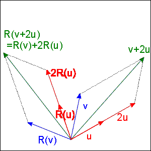Of special interest to us are of course rotations; that these are LTs is obvious geometrically: clearly scaling and adding vectors and then rotating them is the same as first rotating and then scaling and adding them (see Figure 3.1).

Figure 3.1

Problem 3.1. Are translations LTs?

3.2 Matrices of Linear Transformations

Any LT from vector space V to W is completely determined by what it does to any basis for V. For example, suppose we have a LT, called L, from R³ to R². Any such LT is uniquely specified by what it does to the standard basis vectors e₁, e₂ and e₃. To see why, note that if v is any vector in R³, then v can be written in the form v₁e₁ + v₂e₂ + v₃e₃. Then by Formula (3.1), L(v) = v₁L(e₁) + v₂L(e₂) + v₃L(e₃). That is, if we know L(e₁), L(e₂) and L(e₃), we can determine L(v) for all v in R³. Note that this is not true for functions in general. For nonlinear functions, we can know what the function does to all the basis vectors and still have no idea what it does to any other vector. But for a LT acting on an n-D space, we need only know what it does to n basis vectors, and we automatically know everything about the LT. We can use this fact to develop an efficient technique for computing with LTs.

We shall consider a LT, called A this time, and write A_ij for the i^th component (relative to the basis for the output space) of A(e_j), where e_j is the j^th basis vector for the input space V. Thus if the input space is n-D, the index j takes the integer values from 1 to n, because there are n basis vectors e₁, e₂, ..., e_n. Similarly, if the output space is m-D, the index i takes the values from 1 to m, because the vectors A(e_j) in the output space have m components. Thus there are m x n numbers A_ij in total. The vector A(e_j) is called the image under A of the vector e_j, because it's what comes out when you input e_j to A. For example, A₁₂ is the first component of A(e₂), the image under A of e₂. Given any vector v in V, we know from Formula (3.1) that its image, A(v), equals the vector sum v₁A(e₁) + ... + v_nA(e_n). Since vectors are added component-wise, it follows that the first component of A(v) is the sum of the first components of the vectors in this sum; that is, the first component of A(v) is

v₁A₁₁ + ... + v_nA_1n. (3.2)

Similarly, the second component of A(v) is A₂₁v₁ + ... + A_2nv_n (here we have switched the order of the A's and v's in the addends). And in general, for an arbitrary LT, A, the i^th component of A(v) is

A_i1v₁ + ... + A_inv_n (3.3)

Thus if we know the numbers A_ij, we can compute the output of the LT A for any input vector v.

It is convenient to write the numbers A_ij in a rectangular array, called [A], in such a way that A_ij -- the i^th component of A(e_j) -- is the element in the i^th row and j^th column of [A]. Note that the j^th column of [A] is then the vector A(e_j). This array [A] is called the matrix of the LT A relative to the bases chosen for the input and output spaces; if we chose a different basis for either the input or output space, a different matrix would correspond to the same LT A. But notice that any matrix for a LT from an m-D space to an n-D space will always have m columns (one for each basis vector in the input space) and n rows (one for each component of the output vectors in the output space). A matrix with n rows and m columns is called an n by m matrix.

Vectors can be written as n by 1, column matrices: we simply write the n components of the vector v (relative, as always, to some basis) in a column. Recall that the j^th column of [A] is the vector A(e_j). Thus we can construct the matrix of A by writing the m vectors A(e_j) (ie the m images under A of the m basis vectors e_j of the input space) side by side in m columns. And conversely, by inspecting the matrix of A, we can see automatically what A does to the basis vectors.

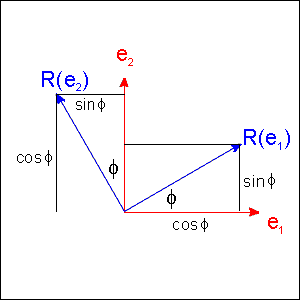
Example 3.1 A rotation, R, of Ø° = 30° counterclockwise in 2-D space takes e₁ to R(e₁) = cosØe₁ + sinØe₂ = (.87, .5) and e₂ to R(e₂) = -sinØe₁ + cosØe₂ = (-.5, .87)

Figure 3.2

Therefore the matrix of this rotation relative to the basis <e₁, e₂> - this is the basis for both the input and output spaces, which are the same 2-D plane - is built by writing the two image vectors R(e₁) and R(e₂) side by side as columns:

Problem 3.2. Find the matrix, relative to the standard basis <e₁, e₂, e₃> for 3-D space, for a 30° leftward rotation about a vertical axis (aligned with e₃).

3.3 Matrix Algebra

There are a number of operations on matrices which have been defined expressly to facilitate calculations with LTs. Taking a few moments now to learn these operations will greatly simplify our later work. The first operation is matrix addition: we can add matrices with the same numbers of rows and columns by adding corresponding elements; that is, if [A], [B] and [C] are matrices, all with m rows and n columns, and [C] = [A] + [B], then

C_ij = A_ij + B_ij (3.4)

The second operation is multiplication of a matrix by a scalar: If A is any matrix and s is any scalar, then the product s[A] is obtained by multiplying each element of [A] by s.

The third operation, and the most important, is matrix multiplication. If [B] is an m by r matrix and [A] is an r by n matrix (note that the number of columns of [B] must equal the number of rows of [A]), then the matrix product [B][A] is an m by n matrix [C] with elements

C_ij = B_i1A_1j + B_i2A_2j + ... + B_irA_rj (3.5)

That is, if you want to compute C_ij, the element in the i^th row and j^th column of [C], you look at the i^th row of [B] and the j^th column of [A]; you multiply the first element of the row with the first element of the column, the second element of the row with the second element of the column, and so on to the end of the row and column, and you add these products together to get C_ij. Note that if you think of the i^th row of B as a vector, (B_i1, B_i2, ... , B_ir), and the j^th column of [A] as another vector, (A_1j, A_2j, ... , A_rj), then Formula (3.5) for C₁₃ looks like Formula (2.2) for the dot product of these two vectors. There is the difference that Formula (2.2), for dot products, is valid only in an orthonormal coordinate system, whereas (3.5), for matrix products, works in any coordinates, but this distinction will not be very important for you since you will almost always be working with orthonormal bases.

Example 3.2. Here is an example of a matrix product [B][A] = [C]:

For instance, we have C₂₃ (the element in the 2nd row and 3rd column of the rightmost matrix) = B₂₁A₁₃ + B₂₂A₂₃ = (3)(9) + (-8)(6) = 27 - 48 = -21. You check the rest.

3.4 Applications of Matrix Multiplication

I. Matrix multiplication can be used to compute the action of a LT on a vector: In the special case where the righthand matrix in a product is a column matrix -- ie a vector -- Formula (3.5) is the same as Formula (3.3) for evaluating a LT. That is, if [A] and [v] are the matrices for a LT and a vector, then [A(v)] (the square brackets emphasize that we are treating this vector as a column matrix) is the matrix product of [A] and [v]:

[A(v)] = [A][v]. (3.6)

Example 3.3. Use the matrix [R] from Example 3.1 to put the vectors (1, 0), (0, 1) and (2, -1) through a 30° counterclockwise rotation.

Solution: To rotate these vectors, we write them as column matrices and multiply by [R]:

The first two calculations simply confirm what we already knew: that the transformed basis vectors are the columns of the matrix. The third computation is a step into the unknown; you should draw a picture to convince yourself that the vector (2.24, .13) really is (2, -1) rotated 30° counterclockwise.

Problem 3.3. Use the matrix from Problem 3.2 to rotate the vector (4, -1, 2) 30° left.

II. Matrix multiplication can be used to compute compositions of LTs: Suppose now that B is a second LT, whose input space is the output space of A. We write B ° A for the composition of B and A (ie A is applied to a vector and then B is applied to the result -- if you wish, you may prove that the composition of LTs is itself a LT). How can we compute what this composite function does to a vector v? We compute first the action of A on v by matrix multiplication: [A(v)] = [A][v], and then we compute the action of B on A(v) by multiplying this output vector by the matrix [B]: [(B ° A)(v)] = [B]([A][v]). It can be shown that matrix multiplication is associative -- ie placement of parenthesis is irrelevant -- so we could equally well multiply the two matrices [B] and [A] together and then multiply [v] by this matrix product [B][A]: [(B ° A)(v)] = ([[B][A])[v]. In other words, the matrix of B ° A is the matrix product [B][A]:

[ B ° A ] = [B][A] (3.7)

An important fact about matrix multiplication is that, even if both products [B][A] and [A][B] are defined, it is not usually the case that [B][A] = [A][B]; that is, matrix multiplication is not commutative. This property reflects the corresponding property of LTs, that composition of LTs in not commutative -- ie LT A followed by B yields a different overall LT, usually, than does B followed by A. It is therefore important to remember that the left to right order of the factors in the matrix multiplication is opposite the order of action of the LTs: if A occurs first and B second, we write the overall function as B ° A, and the corresponding matrix is [B][A]. Problem 3.4 below will give you some practice with LT composition.

3.5 More Matrix Algebra!

The following additional ideas from matrix algebra will also be useful. The n by n identity matrix [I] is the n by n matrix with 1's along the main diagonal and 0's elsewhere. For example, the 3 by 3 identity matrix is

1	0	0
0	1	0
0	0	1

The n by n matrix [I] represents the identity LT, I, on n-D space, which takes every vector to itself: I(v) = v. Formula (3.5) shows that the matrix I times any compatible matrix A yields A: IA = AI = A. (From now on, we'll often reduce the clutter in our matrix formulas by dropping the square brackets and simply writing "I" and "A" for "[I]" and "[A]" etc.; brackets will be used only when we want to emphasize the distinction between a LT and its corresponding matrix).

Any given n by n (ie square) matrix A may or may not have an inverse matrix A^-1, with the property that AA^-1 = A^-1A = I. If A has an inverse, A is called invertible or nonsingular. If A is invertible, then the inverse matrix is unique ie no matrix has two different inverses. If A is the matrix of a LT, L, then A^-1 is the matrix of the inverse LT L^-1 which "undoes" L. If the matrix has no inverse, it means that the corresponding LT is not invertible; that is, given an output, it is not possible to determine what the input to the LT was. A simple example of a noninvertible LT is the one that transforms any input into the zero vector. If I tell you that this LT has given 0 as output, you cannot determine what the input was, because any one of infinitely many different input vectors would have given the same output.

The transpose A^T of a matrix is obtained by interchanging the rows and columns of A, so that the element in the i^th row and j^th column of A is in the j^th row and i^th column of A^T.

The following are the main properties of the matrix product:

MP1. AB is not equal to BA
MP2. A(B + C) = AB + AC
MP3. s(AB) = (sA)B = A(sB)
MP4. (AB)C = A(BC)
MP5. (AB)^-1 = B^-1A^-1
MP6. (AB)^T = B^TA^T

MP1 and MP4 express the noncommutativity and the associativity, respectively, of matrix multiplication, both of which were mentioned in Section 3.4 above. I have stated the rules MP1-6 compactly for easy reference; I assume you will understand them despite some logical shortcuts. For example, you are to understand that the equations in MP2-6 are true for any matrices A, B and C for which the relevant operations are defined. In contrast, MP1 does not mean that AB and BA are always different whenever the products are defined, but only that that they may be (and usually are) different.
OMNIVOR contains the following subprograms for handling matrices: MATMULT multiplies two matrices together, MATVECT multiplies a vector by a matrix, MATINV computes the inverse of a matrix if there is an inverse, and MATTRANSPOSE does what you would expect.

Problem 3.4. Find the matrices relative to the standard orthonormal basis for 3-D space for i. A 60° rightward rotation; ii. A 45° downward rotation; iii. The overall rotation produced by rotating first 60° right and then 45° down (write a program using subprogram MATMULT). What does this overall rotation do to the vector (1, 1, 1) (Use subprogram MATVECT)?

Problem 3.5. Below is the VOR matrix of an experimental subject. Assume that this subject's VOR is pefectly linear, so that the matrix is an exact description of the input-output properties of the reflex. What is the eye velocity output when the head velocity is (1, 0, -2)? What head velocity evokes an eye velocity response of (-1, 3, 7)?

Problem 3.6. Even when we fit the VOR as a nonlinear function of head velocity, we still use matrices, because we represent the VOR as a linear function of something other than simple head velocity . For example, in fitting eye velocity e as a quadratic function of head velocity h, we use a subprogram which tells OMNIVOR that the input to the VOR is not simply head velocity but a 10-component vector x = (1, h₁, h₂, h₃, h₁h₁ / 100, h₁h₂ / 100, h₁h₃ / 100, h₂h₂ / 100, h₂h₃ / 100, h₃h₃ / 100), where h₁, h₂, and h₃ are the torsional, vertical and horizontal components of head velocity. (The last six elements are divided by 100 to keep them from getting unreasonably big; eg when head velocity is 150° / s left, then h₃h₃ = 150² = 22500, but h₃h₃ / 100 is 225, which is not much larger than h₃ itself). OMNIVOR then samples a few thousand pairs of eye and head velocities and finds the 3 by 10 matrix, call it M, that best relates e and x. In other words, M is, of all possible 3 by 10 matrices, the one that makes Mx the best approximation to e. Below is a made-up M matrix (it looks unfamiliar because you are used to seeing these matrices on their sides, in "transpose array", with spaces inserted after the 1st, 4th and 7th lines for clarity). Use this matrix to compute, by hand, the eye velocity output of the VOR when head velocity is (0, 0, 0) and when it's (1, 10, 10).